Upwards and downwards accumulations

Continuing my work in regress, this post revisits—with the benefit of much hindsight—what I was working on for my DPhil thesis (which was summarized in a paper at MPC 1992) and in subsequent papers at MPC 1998 and in SCP in 2000. This is the topic of accumulations on data structures, which distribute information across the data structure. List instances are familiar from the Haskell standard libraries (and, to those with a long memory, from APL); my thesis presented instances for a variety of tree datatypes; and the later work was about making it datatype-generic. I now have a much better way of doing it, using Conor McBride’s derivatives.

Accumulations

Accumulations or scans distribute information contained in a data structure across that data structure in a given direction. The paradigmatic example is computing the running totals of a list of numbers, which can be thought of as distributing the numbers rightwards across the list, summing them as you go. In Haskell, this is an instance of the {\mathit{scanl}} operator:

\displaystyle  \begin{array}{lcl} \mathit{scanl} &::& (\beta \rightarrow \alpha \rightarrow \beta) \rightarrow \beta \rightarrow [\alpha] \rightarrow [\beta] \\ \mathit{scanl}\,f\,e\,[\,] &=& [e] \\ \mathit{scanl}\,f\,e\,(a:x) &=& e : \mathit{scanl}\,f\,(f\,e\,a)\,x \medskip \\ \mathit{totals} &::& [{\mathbb Z}] \rightarrow [{\mathbb Z}] \\ \mathit{totals} &=& \mathit{scanl}\,(+)\,0 \end{array}

A special case of this pattern is to distribute the elements of a list rightwards across the list, simply collecting them as you go, rather than summing them. That’s the {\mathit{inits}} function, and it too is an instance of {\mathit{scanl}}:

\displaystyle  \mathit{inits} = \mathit{scanl}\,\mathit{snoc}\,[\,] \quad\mathbf{where}\; \mathit{snoc}\,x\,a = x \mathbin{{+}\!\!\!{+}} [a]

It’s particularly special, in the sense that it is the most basic {\mathit{scanl}}; any other instance can be expressed in terms of it:

\displaystyle  \mathit{scanl}\,f\,e = \mathit{map}\,(\mathit{foldl}\,f\,e) \cdot \mathit{inits}

This is called the Scan Lemma for {\mathit{scanl}}. Roughly speaking, it states that a {\mathit{scanl}} replaces every node of a list with a {\mathit{foldl}} applied to that node’s predecessors. Read from right to left, the scan lemma is an efficiency-improving transformation, eliminating duplicate computations; but note that this only works on expressions {\mathit{map}\,f \cdot \mathit{inits}} where {f} is a {\mathit{foldl}}, because only then are there duplicate computations to eliminate. It’s an important result, because it relates a clear and simple specification on the right to a more efficient implementation on the left.

However, the left-to-right operators {\mathit{inits}}, {\mathit{foldl}}, and {\mathit{scanl}} are a little awkward in Haskell, because they go against the grain of the cons-based (ie, right-to-left) structure of lists. I leave as a simple exercise for the reader the task of writing the more natural {\mathit{tails}}, {\mathit{foldr}}, and {\mathit{scanr}}, and identifying the relationships between them. Conversely, one can view {\mathit{inits}} etc as the natural operators for snoc-based lists, which are constructed from nil and snoc rather than from nil and cons.

Upwards and downwards accumulations on binary trees

What would {\mathit{inits}}, {\mathit{tails}}, {\mathit{scanl}}, etc look like on different—and in particular, non-linear—datatypes? Let’s consider a simple instance, for homogeneous binary trees; that is, trees with a label at both internal and external nodes.

\displaystyle  \mathbf{data}\;\mathsf{Tree}\,\alpha = \mathit{Leaf}\,\alpha \mid \mathit{Fork}\,\alpha\,(\mathsf{Tree}\,\alpha)\,(\mathsf{Tree}\,\alpha)

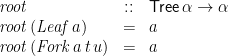
for which the obvious fold operator is

\displaystyle  \begin{array}{lcl} \mathit{fold} &::& (\alpha\rightarrow\beta) \rightarrow (\alpha\rightarrow\beta\rightarrow\beta\rightarrow\beta) \rightarrow \mathsf{Tree}\,\alpha \rightarrow \beta \\ \mathit{fold}\,f\,g\,(\mathit{Leaf}\,a) &=& f\,a \\ \mathit{fold}\,f\,g\,(\mathit{Fork}\,a\,t\,u) &=& g\,a\,(\mathit{fold}\,f\,g\,t)\,(\mathit{fold}\,f\,g\,u) \end{array}

I’m taking the view that the appropriate generalization is to distribute data “upwards” and “downwards” through such a tree—from the leaves towards the root, and vice versa. This does indeed specialize to the definitions we had on lists when you view them vertically in terms of their “cons” structure: they’re long thin trees, in which every parent has exactly one child. (An alternative view would be to look at distributing data horizontally through a tree, from left to right and vice versa. Perhaps I’ll come back to that another time.)

The upwards direction is the easier one to deal with. An upwards accumulation labels every node of the tree with some function of its descendants; moreover, the descendants of a node themselves form a tree, so can be easily represented, and folded. So we can quite straightforwardly define:

\displaystyle  \begin{array}{lcl} \mathit{scanu} &::& (\alpha\rightarrow\beta) \rightarrow (\alpha\rightarrow\beta\rightarrow\beta\rightarrow\beta) \rightarrow \mathsf{Tree}\,\alpha \rightarrow \mathsf{Tree}\,\beta \\ \mathit{scanu}\,f\,g\,(\mathit{Leaf}\,a) &=& \mathit{Leaf}\,(f\,a) \\ \mathit{scanu}\,f\,g\,(\mathit{Fork}\,a\,t\,u) &=& \mathit{Fork}\,(g\,a\,(\mathit{root}\,t')\,(\mathit{root}\,u'))\,t'\,u' \\ & & \quad\mathbf{where}\; t' = \mathit{scanu}\,f\,g\,t ; u' = \mathit{scanu}\,f\,g\,u \end{array}

where {\mathit{root}} yields the root of a tree:

\displaystyle  \begin{array}{lcl} \mathit{root} &::& \mathsf{Tree}\,\alpha \rightarrow \alpha \\ \mathit{root}\,(\mathit{Leaf}\,a) &=& a \\ \mathit{root}\,(\mathit{Fork}\,a\,t\,u) &=& a \end{array}

As with lists, the most basic upwards scan uses the constructors themselves as arguments:

\displaystyle  \begin{array}{lcl} \mathit{subtrees} &::& \mathsf{Tree}\,\alpha \rightarrow \mathsf{Tree}\,(\mathsf{Tree}\,\alpha) \\ \mathit{subtrees} &=& \mathit{scanu}\,\mathit{Leaf}\,\mathit{Fork} \end{array}

and any other scan can be expressed, albeit less efficiently, in terms of this:

\displaystyle  \mathit{scanu}\,f\,g = \mathit{fmap}\,(\mathit{fold}\,f\,g) \cdot \mathit{subtrees}

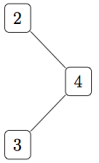
The downwards direction is more difficult, though. A downwards accumulation should label every node with some function of its ancestors; but these do not form another tree. For example, in the homogeneous binary tree

the ancestors of the node labelled {3} are the nodes labelled {2,4,3}. One could represent those ancestors simply as a list, {[2,4,3]}; but that rules out the possibility of a downwards accumulation treating left children differently from right children, which is essential in a number of algorithms (such as the parallel prefix and tree drawing algorithms in my thesis). A more faithful rendering is to define a new datatype of paths that captures the left and right turns—a kind of non-empty cons list, but with both a “left cons” and a “right cons” constructor:

\displaystyle  \mathbf{data}\;\mathsf{Path}\,\alpha = \mathit{Single}\,\alpha \mid \mathit{LCons}\,\alpha\,(\mathsf{Path}\,\alpha) \mid \mathit{RCons}\,\alpha\,(\mathsf{Path}\,\alpha)

(I called them “threads” in my thesis.) Then we can capture the data structure representing the ancestors of the node labelled {3}

by the expression {\mathit{RCons}\,2\,(\mathit{LCons}\,4\,(\mathit{Single}\,3))}. I leave it as an exercise for the more energetic reader to work out a definition for

\displaystyle  \mathit{paths} :: \mathsf{Tree}\,\alpha \rightarrow \mathsf{Tree}\,(\mathsf{Path}\,\alpha)

to compute the tree giving the ancestors of every node, and for a corresponding {\mathit{scand}}.

Generic upwards accumulations

Having seen ad-hoc constructions for a particular kind of binary tree, we should consider what the datatype-generic construction looks like. I discussed datatype-generic upwards accumulations already, in the post on Horner’s Rule; the construction was given in the paper Generic functional programming with types and relations by Richard Bird, Oege de Moor and Paul Hoogendijk. As with homogeneous binary trees, it’s still the case that the generic version of {\mathit{subtrees}} labels every node of a data structure of type {\mathsf{T}\alpha = \mu\mathsf{F}\alpha} with the descendants of that node, and still the case that the descendants form a data structure also of type {\mathsf{T}\alpha}. However, in general, the datatype {\mathsf{T}} does not allow for a label at every node, so we need the labelled variant {\mathsf{L}\alpha = \mu\mathsf{G}\alpha} where {\mathsf{G}(\alpha,\beta) = \alpha \times \mathsf{F}(1,\beta)}. Then we can define

\displaystyle  \mathit{subtrees}_{\mathsf{F}} = \mathit{fold}_{\mathsf{F}}(\mathit{in}_{\mathsf{G}} \cdot \mathit{fork}(\mathit{in}_{\mathsf{F}} \cdot \mathsf{F}(\mathit{id},\mathit{root}), \mathsf{F}(!,\mathit{id}))) :: \mathsf{T}\alpha \rightarrow \mathsf{L}(\mathsf{T}\alpha)

where {\mathit{root} = \mathit{fst} \cdot \mathit{in}_{\mathsf{G}}^{-1} = \mathit{fold}_{\mathsf{G}}\,\mathit{fst} :: \mathsf{L}\alpha \rightarrow \alpha} returns the root label of a labelled data structure—by construction, every labelled data structure has a root label—and {!_{\alpha} :: \alpha \rightarrow 1} is the unique arrow to the unit type. Moreover, we get a datatype-generic {\mathit{scanu}} operator, and a Scan Lemma:

\displaystyle  \begin{array}{lcl} \mathit{scanu}_{\mathsf{F}} &::& (\mathsf{F}(\alpha,\beta) \rightarrow \beta) \rightarrow \mathsf{T}\alpha \rightarrow \mathsf{L}\beta \\ \mathit{scanu}_{\mathsf{F}}\,\phi &=& \mathsf{L}\,(\mathit{fold}_{\mathsf{F}}\,\phi) \cdot \mathit{subtrees}_{\mathsf{F}} \\ &=& \mathit{fold}_{\mathsf{F}}(\mathit{in}_{\mathsf{G}} \cdot \mathit{fork}(\phi \cdot \mathsf{F}(\mathit{id},\mathit{root}), \mathsf{F}(!,\mathit{id}))) \end{array}

Generic downwards accumulations, via linearization

The best part of a decade after my thesis work, inspired by the paper by Richard Bird & co, I set out to try to define datatype-generic versions of downward accumulations too. I wrote a paper about it for MPC 1998, and then came up with a new construction for the journal version of that paper in SCP in 2000. I now think these constructions are rather clunky, and I have a better one; if you don’t care to explore the culs-de-sac, skip this section and the next and go straight to the section on derivatives.

The MPC construction was based around a datatype-generic version of the {\mathsf{Path}} datatype above, to represent the “ancestors” of a node in an inductive datatype. The tricky bit is that data structures in general are non-linear—a node may have many children—whereas paths are linear—every node has exactly one child, except the last which has none; how can we define a “linear version” {\mathsf{F}'} of {\mathsf{F}}? Technically, we might say that a functor is linear (actually, “affine” would be a better word) if it distributes over sum.

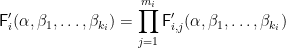
The construction in the paper assumed that {\mathsf{F}} was a sum of products of literals

\displaystyle  \begin{array}{lcl} \mathsf{F}(\alpha,\beta) &=& \sum_{i=1}^{n} \mathsf{F}_i(\alpha,\beta) \\ \mathsf{F}_i(\alpha,\beta) &=& \prod_{j=1}^{m_i} \mathsf{F}_{i,j}(\alpha,\beta) \end{array}

where each {\mathsf{F}_{i,j}(\alpha,\beta)} is either {\alpha}, {\beta}, or some constant type such as {\mathit{Int}} or {\mathit{Bool}}. For example, for leaf-labelled binary trees

\displaystyle  \mathbf{data}\;\mathsf{Tree}\,\alpha = \mathit{Tip}\,\alpha \mid \mathit{Bin}\,(\mathsf{Tree}\,\alpha)\,(\mathsf{Tree}\,\alpha)

the shape functor is
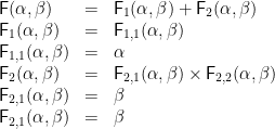
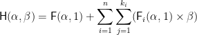
 {\mathsf{F}(\alpha,\beta) = \alpha + \beta \times \beta}, so {n=2} (there are two variants), {m_1=1} (the first variant has a single literal, {\alpha}) and {m_2=2} (the second variant has two literals, {\beta} and {\beta}), and:

\displaystyle  \begin{array}{lcl} \mathsf{F}(\alpha,\beta) &=& \mathsf{F}_1(\alpha,\beta) + \mathsf{F}_2(\alpha,\beta) \\ \mathsf{F}_1(\alpha,\beta) &=& \mathsf{F}_{1,1}(\alpha,\beta) \\ \mathsf{F}_{1,1}(\alpha,\beta) &=& \alpha \\ \mathsf{F}_2(\alpha,\beta) &=& \mathsf{F}_{2,1}(\alpha,\beta) \times \mathsf{F}_{2,2}(\alpha,\beta) \\ \mathsf{F}_{2,1}(\alpha,\beta) &=& \beta \\ \mathsf{F}_{2,1}(\alpha,\beta) &=& \beta \\ \end{array}

Then for each {i} we define a {(k_i+1)}-ary functor {\mathsf{F}'_i}, where {k_i} is the “degree of branching” of variant {i} (ie, the number of {\beta}s occurring in {\mathsf{F}_i(\alpha,\beta)}, which is the number of {j} for which {\mathsf{F}_{i,j}(\alpha,\beta)=\beta}), in such a way that

\displaystyle  \mathsf{F}'_i(\alpha,\beta,\ldots,\beta) = \mathsf{F}_i(\alpha,\beta)

and {\mathsf{F}'_i} is linear in each argument except perhaps the first. It’s a bit messy explicitly to give a construction for {\mathsf{F}'_i}, but roughly speaking,

\displaystyle  \mathsf{F}'_i(\alpha,\beta_1,\ldots,\beta_{k_i}) = \prod_{j=1}^{m_i} \mathsf{F}'_{i,j}(\alpha,\beta_1,\ldots,\beta_{k_i})

where {\mathsf{F}'_{i,j}(\alpha,\beta_1,\ldots,\beta_{k_i})} is “the next unused {\beta_i}” when {\mathsf{F}_{i,j}(\alpha,\beta)=\beta}, and just {\mathsf{F}_{i,j}(\alpha,\beta)} otherwise. For example, for leaf-labelled binary trees, we have:

\displaystyle  \begin{array}{lcl} \mathsf{F}'_1(\alpha) &=& \alpha \\ \mathsf{F}'_2(\alpha,\beta_1,\beta_2) &=& \beta_1 \times \beta_2 \end{array}

Having defined the linear variant {\mathsf{F}'} of {\mathsf{F}}, we can construct the datatype {\mathsf{P}\alpha = \mu\mathsf{H}\alpha} of paths, as the inductive datatype of shape {\mathsf{H}} where

\displaystyle  \mathsf{H}(\alpha,\beta) = \mathsf{F}(\alpha,1) + \sum_{i=1}^{n} \sum_{j=1}^{k_i} (\mathsf{F}_i(\alpha,1) \times \beta)

That is, paths are a kind of non-empty cons list. The path ends at some node of the original data structure; so the last element of the path is of type {\mathsf{F}(\alpha,1)}, which records the “local content” of a node (its shape and labels, but without any of its children). Every other element of the path consists of the local content of a node together with an indication of which direction to go next; this amounts to the choice of a variant {i}, followed by the choice of one of {k_i} identical copies of the local contents {\mathsf{F}_i(\alpha,1)} of variant {i}, where {k_i} is the degree of branching of variant {i}. We model this as a base constructor {\mathit{End}} and a family of “cons” constructors {\mathit{Cons}_{i,j}} for {1 \le i \le n} and {1 \le j \le k_i}.

For example, for leaf-labelled binary trees, the “local content” for the last element of the path is either a single label (for tips) or void (for bins), and for the other path elements, there are zero copies of the local content for a tip (because a tip has zero children), and two copies of the void local information for bins (because a bin has two children). Therefore, the path datatype for such trees is

\displaystyle  \mathbf{data}\;\mathsf{Path}\,\alpha = \mathit{End}\,(\mathsf{Maybe}\,\alpha) \mid \mathit{Cons}_{2,1}\,(\mathsf{Path}\,\alpha) \mid \mathit{Cons}_{2,2}\,(\mathsf{Path}\,\alpha)

which is isomorphic to the definition that you might have written yourself:

\displaystyle  \mathbf{data}\;\mathsf{Path}\,\alpha = \mathit{External}\,\alpha \mid \mathit{Internal} \mid \mathit{Left}\,(\mathsf{Path}\,\alpha) \mid \mathit{Right}\,(\mathsf{Path}\,\alpha)

For homogeneous binary trees, the construction gives

\displaystyle  \mathbf{data}\;\mathsf{Path}\,\alpha = \mathit{External}\,\alpha \mid \mathit{Internal}\,\alpha \mid \mathit{Left}\,\alpha\,(\mathsf{Path}\,\alpha) \mid \mathit{Right}\,\alpha\,(\mathsf{Path}\,\alpha)

which is almost the ad-hoc definition we had two sections ago, except that it distinguishes singleton paths that terminate at an external node from those that terminate at an internal one.

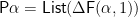
Now, analogous to the function {\mathit{subtrees}_\mathsf{F}} which labels every node with its descendants, we can define a function {\mathit{paths}_\mathsf{F} : \mathsf{T}\alpha \rightarrow \mathsf{L}(\mathsf{P}\alpha)} to label every node with its ancestors, in the form of the path to that node. One definition is as a fold; informally, at each stage we construct a singleton path to the root, and map the appropriate “cons” over the paths to each node in each of the children (see the paper for a concrete definition). This is inefficient, because of the repeated maps; it’s analogous to defining {\mathit{inits}} by

\displaystyle  \begin{array}{lcl} \mathit{inits}\,[\,] &=& [[\,]] \\ \mathit{inits}\,(a:x) &=& [\,] : \mathit{map}\,(a:)\,(\mathit{inits}\,x) \end{array}

A second definition is as an unfold, maintaining as an accumulating parameter of type {\mathsf{P}(\alpha)\rightarrow\mathsf{P}(\alpha)} the “path so far”; this avoids the maps, but it is still quadratic because there are no common subexpressions among the various paths. (This is analogous to an accumulating-parameter definition of {\mathit{inits}}:

\displaystyle  \begin{array}{lcl} \mathit{inits} &=& \mathit{inits}'\,\mathit{id} \medskip \\ \mathit{inits}'\,f\,[\,] &=& f\,[\,] \\ \mathit{inits}'\,f\,(a:x) &=& f\,[\,] : \mathit{inits}'\,(f \cdot (a:))\,x \end{array}

Even with an accumulating “Hughes list” parameter, it still takes quadratic time.)

The downwards accumulation itself is defined as a path fold mapped over the paths, giving a Scan Lemma for downwards accumulations. With either the fold or the unfold definition of paths, this is still quadratic, again because of the lack of common subexpressions in a result of quadratic size. However, in some circumstances the path fold can be reassociated (analogous to turning a {\mathit{foldr}} into a {\mathit{foldl}}), leading finally to a linear-time computation; see the paper for the details of how.

Generic downwards accumulations, via zip

I was dissatisfied with the “…”s in the MPC construction of datatype-generic paths, but couldn’t see a good way of avoiding them. So in the subsequent SCP version of the paper, I presented an alternative construction of downwards accumulations, which does not go via a definition of paths; instead, it goes directly to the accumulation itself.

As with the efficient version of the MPC construction, it is coinductive, and uses an accumulating parameter to carry in to each node the seed from higher up in the tree; so the downwards accumulation is of type {\gamma \times \mathsf{T}\alpha \rightarrow \mathsf{L}\beta}. It is defined as an unfold, with a body {g} of type

\displaystyle  \gamma \times \mathsf{T}\alpha \rightarrow \mathsf{G}(\beta, \gamma \times \mathsf{T}\alpha)

The result {\mathsf{G}(\beta, \gamma \times \mathsf{T}\alpha)} of applying the body will be constructed from two components, of types {\mathsf{G}(\beta, \gamma)} and {\mathsf{G}(1, \mathsf{T}\alpha)}: the first gives the root label of the accumulation and the seeds for processing the children, and the second gives the children themselves.

These two components get combined to make the whole result via a function

\displaystyle  \mathit{zip} :: \mathsf{G}(\alpha,\beta) \times \mathsf{G}(\gamma,\delta) \rightarrow \mathsf{G}(\alpha \times \gamma, \beta \times \delta)

This will be partial in general, defined only for pairs of {\mathsf{G}}-structures of the same shape.

The second component of {g} is the easier to define; given input {\gamma \times \mathsf{T}\alpha}, it unpacks the {\mathsf{T}\alpha} to {\mathsf{F}(\alpha,\mathsf{T}\alpha)}, and discards the {\gamma} and the {\alpha} (recall that {\mathsf{L}\alpha=\mu\mathsf{G}\alpha} is the labelled variant of {\mathsf{T}\alpha=\mu\mathsf{F}\alpha}, where {\mathsf{G}(\alpha,\beta) = \alpha \times \mathsf{F}(1,\beta)}).

For the first component, we enforce the constraint that all output labels are dependent only on their ancestors by unpacking the {\mathsf{T}\alpha} and pruning off the children, giving input {\gamma \times \mathsf{F}(\alpha,1)}. We then suppose as a parameter to the accumulation a function {f} of type {\gamma \times \mathsf{F}(\alpha,1) \rightarrow \beta \times \mathsf{F}(1,\gamma) = \mathsf{G}(\beta,\gamma)} to complete the construction of the first component. In order that the two components can be zipped together, we require that {f} is shape-preserving in its second argument:

\displaystyle  \mathsf{F}(!,!) \cdot \mathit{snd} = \mathsf{F}(!,!) \cdot f \cdot \mathit{snd}

where {! : \alpha \rightarrow 1} is the unique function to the unit type. Then, although the {g} built from these two components depends on the partial function {\mathit{zip}}, it will still itself be total.

The SCP construction gets rid of the “…”s in the MPC construction. It is also inherently efficient, in the sense that if the core operation {f} takes constant time then the whole accumulation takes linear time. However, use of the partial {\mathit{zip}} function to define a total accumulation is a bit unsatisfactory, taking us outside the domain of sets and total functions. Moreover, there’s now only half an explanation in terms of paths: accumulations in which the label attached to each node depends only on the list of its ancestors, and not on the left-to-right ordering of siblings, can be factored into a list function (in fact, a {\mathit{foldl}}) mapped over the “paths”, which is now a tree of lists; but accumulations in which left children are treated differently from right children, such as the parallel prefix and tree drawing algorithms mentioned earlier, can not.

Generic downwards accumulations, via derivatives

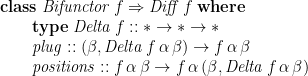
After another interlude of about a decade, and with the benefit of new results to exploit, I had a “eureka” moment: the linearization of a shape functor is closely related to the beautiful notion of the derivative of a datatype, as promoted by Conor McBride. The crucial observation Conor made is that the “one-hole contexts” of a datatype—that is, for a container datatype, the datatype of data structures with precisely one element missing—can be neatly formalized using an analogue of the rules of differential calculus. The one-hole contexts are precisely what you need to identify which particular child you’re talking about out of a collection of children. (If you’re going to follow along with some coding, I recommend that you also read Conor’s paper Clowns to the left of me, jokers to the right. This gives the more general construction of dissecting a datatype, identifying a unique hole, but also allowing the “clowns” to the left of the hole to have a different type from the “jokers” to the right. I think the explanation of the relationship with the differential calculus is much better explained here; the original notion of derivative can be retrieved by specializing the clowns and jokers to the same type.)

The essence of the construction is the notion of a derivative {\Delta\mathsf{F}} of a functor {\mathsf{F}}. For our purposes, we want the derivative in the second argument only of a bifunctor; informally, {\Delta\mathsf{F}(\alpha,\beta)} is like {\mathsf{F}(\alpha,\beta)}, but with precisely one {\beta} missing. Given such a one-hole context, and an element with which to plug the hole, one can reconstruct the whole structure:

\displaystyle  \mathit{plug}_\mathsf{F} :: \beta \times \Delta\mathsf{F}(\alpha,\beta) \rightarrow \mathsf{F}(\alpha,\beta)

That’s how to consume one-hole contexts; how can we produce them? We could envisage some kind of inverse {\mathit{unplug}} of {\mathit{plug}}, which breaks an {\mathsf{F}}-structure into an element and a context; but this requires us to invent a language for specifying which particular element we mean—{\mathit{plug}} is not injective, so {\mathit{unplug}} needs an extra argument. A simpler approach is to provide an operator that annotates every position at once with the one-hole context for that position:

\displaystyle  \mathit{positions}_\mathsf{F} :: \mathsf{F}(\alpha,\beta) \rightarrow \mathsf{F}(\alpha, \beta \times \Delta\mathsf{F}(\alpha,\beta))

One property of {\mathit{positions}} is that it really is an annotation—if you throw away the annotations, you get back what you started with:

\displaystyle  \mathsf{F}(\mathit{id},\mathit{fst})\,(\mathit{positions}\,x) = x

A second property relates it to {\mathit{plug}}—each of elements in a hole position plugs into its associated one-hole context to yield the same whole structure back again:

\displaystyle  \mathsf{F}(\mathit{id},\mathit{plug})\,(\mathit{positions}\,x) = \mathsf{F}(\mathit{id},\mathit{const}\,x)\,x

(I believe that those two properties completely determine {\mathit{plug}} and {\mathit{positions}}.)

Incidentally, the derivative {\Delta\mathsf{F}} of a bifunctor can be elegantly represented as an associated type synonym in Haskell, in a type class {\mathit{Diff}} of bifunctors differentiable in their second argument, along with {\mathit{plug}} and {\mathit{positions}}:

\displaystyle  \begin{array}{lcl} \mathbf{class}\; \mathit{Bifunctor}\,f \Rightarrow \mathit{Diff}\,f \;\mathbf{where} \\ \qquad \mathbf{type}\; \mathit{Delta}\,f :: \ast \rightarrow \ast \rightarrow \ast \\ \qquad \mathit{plug} :: (\beta, \mathit{Delta}\,f\,\alpha\,\beta) \rightarrow f\,\alpha\,\beta \\ \qquad \mathit{positions} :: f\,\alpha\,\beta \rightarrow f\,\alpha\,(\beta, \mathit{Delta}\,f\,\alpha\,\beta) \end{array}

Conor’s papers show how to define instances of {\mathit{Diff}} for all polynomial functors {\mathsf{F}}—anything made out of constants, projections, sums, and products.

The path to a node in a data structure is simply a list of one-hole contexts—let’s say, innermost context first, although it doesn’t make much difference—but with all the data off the path (that is, the other children) stripped away:

\displaystyle  \mathsf{P}\alpha = \mathsf{List}(\Delta\mathsf{F}(\alpha,1))

This is a projection of Huet’s zipper, which preserves the off-path children, and records also the subtree in focus at the end of the path:

\displaystyle  \mathsf{Zipper}_\mathsf{F}\,\alpha = \mathsf{List}(\Delta\mathsf{F}(\alpha,\mu\mathsf{F}\alpha)) \times \mu\mathsf{F}\alpha

Since the contexts are listed innermost-first in the path, closing up a zipper to reconstruct a tree is a {\mathit{foldl}} over the path:

\displaystyle  \begin{array}{lcl} close_\mathsf{F} &::& \mathsf{Zipper}_\mathsf{F}\,\alpha \rightarrow \mu\mathsf{F}\alpha \\ close_\mathsf{F}\,(p,t) &=& \mathit{foldl}\,(\mathit{in}\cdot\mathit{plug})\,t\,p \end{array}

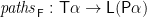
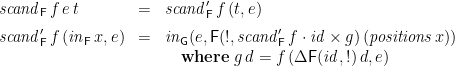
Now, let’s develop the function {\mathit{paths}}, which turns a tree into a labelled tree of paths. We will write it with an accumulating parameter, representing the “path so far”:

\displaystyle  \begin{array}{lcl} \mathit{paths}_\mathsf{F} &::& \mathsf{T}\alpha \rightarrow \mathsf{L}(\mathsf{P}\alpha) \\ \mathit{paths}_\mathsf{F}\,t &=& \mathit{paths}'_\mathsf{F}\,(t,[\,]) \end{array}

Given the components {\mathit{in}_\mathsf{F}\,x} of a tree and a path {p} to its root, {\mathit{paths}'_\mathsf{F}} must construct the corresponding labelled tree of paths. Since {\mathsf{L} = \mu\mathsf{G}} and {\mathsf{G}(\alpha,\beta) = \alpha \times \mathsf{F}(1,\beta)}, this amounts to constructing a value of type {\mathsf{P}\alpha \times \mathsf{F}(1, \mathsf{L}(\mathsf{P}\alpha))}. For the first component of this pair we will use {p}, the path so far. The second component can be constructed from {x} by identifying all children via {\mathit{positions}}, discarding some information with judicious {!}s, consing each one-hole context onto {p} to make a longer path, then making recursive calls on each child:

That is,

\displaystyle  \begin{array}{lcl} \mathit{paths}'_\mathsf{F} &::& \mathsf{T}\alpha\times\mathsf{P}\alpha \rightarrow \mathsf{L}(\mathsf{P}\alpha) \\ \mathit{paths}'_\mathsf{F}\,(\mathit{in}_\mathsf{F}\,x,p) &=& \mathit{in}_\mathsf{G}(p, \mathsf{F}(!, \mathit{paths}'_\mathsf{F} \cdot \mathit{id}\times((:p)\cdot\Delta\mathsf{F}(\mathit{id},!)) )\,(\mathit{positions}\,x)) \end{array}

Downwards accumulations are then path functions mapped over the result of {\mathit{paths}}. However, we restrict ourselves to path functions that are instances of {\mathit{foldr}}, because only then are there common subexpressions to be shared between a parent and its children (remember that paths are innermost-first, so related nodes share a tail of their ancestors).

\displaystyle  \begin{array}{lcl} \mathit{scand}_\mathsf{F} &::& (\Delta\mathsf{F}(\alpha,1)\times\beta\rightarrow\beta) \rightarrow \beta \rightarrow \mathsf{T}\alpha \rightarrow \mathsf{L}\beta \\ \mathit{scand}_\mathsf{F}\,f\,e &=& \mathit{map}\,(\mathit{foldr}\,f\,e) \cdot \mathit{paths} \end{array}

Moreover, it is straightforward to fuse the {\mathit{map}} with {\mathit{paths}}, to obtain

\displaystyle  \begin{array}{lcl} \mathit{scand}_\mathsf{F}\,f\,e\,t &=& \mathit{scand}'_\mathsf{F}\,f\,(t,e) \medskip \\ \mathit{scand}'_\mathsf{F}\,f\,(\mathit{in}_\mathsf{F}\,x,e) &=& \mathit{in}_\mathsf{G}(e, \mathsf{F}(!, \mathit{scand}'_\mathsf{F}\,f \cdot \mathit{id}\times g )\,(\mathit{positions}\,x)) \\ & & \quad\mathbf{where}\; g\,d = f\,(\Delta\mathsf{F}(\mathit{id},!)\,d, e) \end{array}

which takes time linear in the size of the tree, assuming that {f} and {e} take constant time.

Finally, in the case that the function being mapped over the paths is a {\mathit{foldl}} as well as a {\mathit{foldr}}, then we can apply the Third Homomorphism Theorem to conclude that it is also an associative fold over lists. From this (I believe) we get a very efficient parallel algorithm for computing the accumulation, taking time logarithmic in the size of the tree—even if the tree has greater than logarithmic depth.

About jeremygibbons

Jeremy Gibbons is Professor of Computing in Oxford University Department of Computer Science, and a fan of functional programming and patterns of computation.
This entry was posted in Uncategorized. Bookmark the permalink.

2 Responses to Upwards and downwards accumulations

  1. Tom Davies says:

    Isn’t the type of scanl in the first paragraph of code incorrect? That is, the last type should be [alpha] rather than just alpha.

Leave a comment